This post is broken into two parts, written at two different times. In Part 1, I conclude that pre-earnings straddles are not a good investment strategy based on a random sample of 20 companies from the S&P 100. This result is in tension with Capital Market Laboratories which published claims that pre-earnings straddles have an empirical win rate of 60%. To address this discrepancy, in Part 2 I recreate the details of CML's claim using the same index (DOW 30 + NASDAQ 100) and time frame (2012-2017). With these parameters, I find average returns of +2% per straddle but a win rate of just 43%.
Part 1 - 5/13/18
Preliminary Findings
Introduction
A pre-earnings straddle is an options trading strategy comprised of an at-the-money call and an at-the-money put. Since both the call and the put are at-the-money, it is a non-directional strategy aiming to profit off volatility. The strategy is executed by buying the pair of options sometime roughly a week before earnings and selling them just prior to the actual earnings report - the idea being that the increased volatility around earnings is not always accounted for by time decay and you can profit off this without the risk of actually holding positions during earnings. The way you lose, however, is if the time decay of the options price is not offset by unaccounted for volatility.
Post-Selection
Like most get rich quick schemes, I have a hunch that this strategy is too good to be true, despite claims made by Capital Market Laboratories (see here). I believe the reason CML is able to make videos showing empirically tested winning strategies is simply post-selection bias, or the ability to look back on a whole bunch of statistical tests and selectively choose which ones to report (i.e. p-hacking).
For example, if we implement a pre-earnings straddle on the FANG stocks (Facebook, Amazon, Netflix, Google) over the past five years, we find average returns of 56% (shown below).
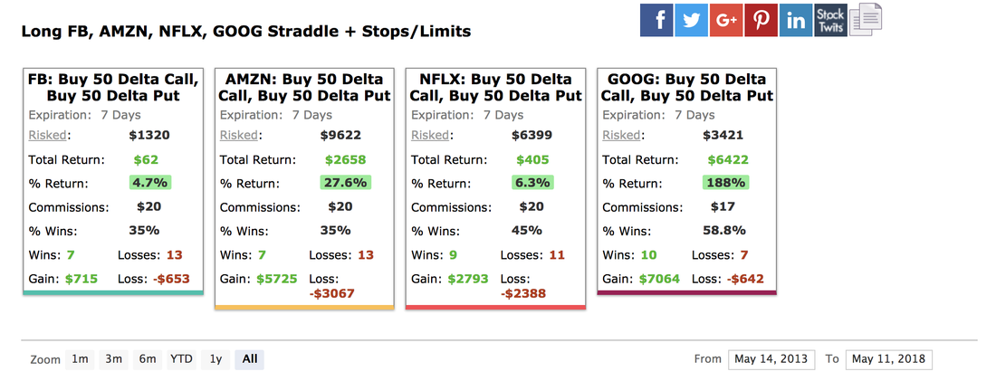
Pre-earnings straddle results for FANG stocks over the past 5 years (data from CML Trade Machine).
However, it is well known that FANG stocks have been some of the best-performing stocks over the past five years and by selecting these stocks we are using our current knowledge of their success to bias the backtest. In cases like this, winning strategies have little to do with empirical evidence and much more to do with the benefit of hindsight.
Backtest
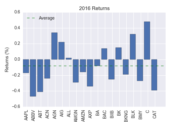
If pre-earnings straddles are indeed a good investment strategy, we should expect them to work, on average, for an unbiased sample of companies. To test this hypothesis, I chose 20 stocks quasi-randomly (alphabetically) from the S&P 100 and backtested a pre-earnings strategy on them for the year 2016. Note, the data for this analysis was downloaded using CML Trade Machine. The year 2016 was chosen randomly from the past five years.
Not surprisingly, I find an average return of -8% (shown below). Not only does the strategy not beat the market, it actually lost money!
Backtest
If pre-earnings straddles are indeed a good investment strategy, we should expect them to work, on average, for an unbiased sample of companies. To test this hypothesis, I chose 20 stocks quasi-randomly (alphabetically) from the S&P 100 and backtested a pre-earnings strategy on them for the year 2016. Note, the data for this analysis was downloaded using CML Trade Machine. The year 2016 was chosen randomly from the past five years.
Not surprisingly, I find an average return of -8% (shown below). Not only does the strategy not beat the market, it actually lost money!
Pro Scan
In Part 2, I will formally analyze pre-earnings straddles over a much more representative data set but, before doing so, I can use CML Trade Machine's Pro Scan feature to quickly apply a pre-earnings straddle to the entire S&P 500. This feature is meant only to "scan" the market for trends but, in doing so, it appears to provide a rank-ordered list of company win percentage for a given strategy. It also appears to only show win rates above 50%, which means we can use the length of this list to see the number of companies that a given strategy works for. Of course, there is the caveat that a win rate under 50% can still have positive average returns but this method should give us a feel for whether or not these strategies are worthwhile.
As the figure below shows, only 67 companies in the S&P 500 have win rates greater than 50% under pre-earnings straddles over the past three years.
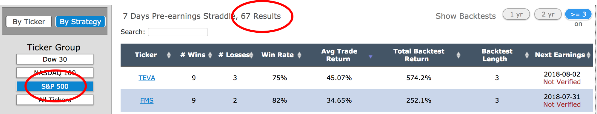
Using the Pro Scan feature to quickly apply a pre-earnings straddle to the S&P 500 yields only 67 winning companies.
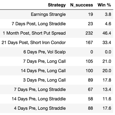
Furthermore, we can quickly repeat this analysis for every possible earnings strategy in CML Trade Machine, which includes an assortment of strangles, straddles, spreads, and calls. As the table below shows, it appears every strategy has a win rate under 50% over the past 3 years for the S&P 500. To me, this implies these strategies are not likely to make money.
Part 2 - 11/10/18
Further Analysis
In Part 1, I backtested a pre-earnings straddle on 20 randomly chosen companies from the S&P 100 in 2016 and found an average return of -8%. In addition, I used the Pro Scan feature to determine what percentage of companies had a win rate over 50% under a variety of strategies. This was not an in-depth analysis, but rather, an effort designed to get a feel for what an in-depth analysis would likely to show. However, due to public scrutiny, the time has come to perform a more thorough analysis - the goal of which is to formally address the claim from CMLviz that pre-earnings straddles have a 60% win rate over the past six years (shown below).
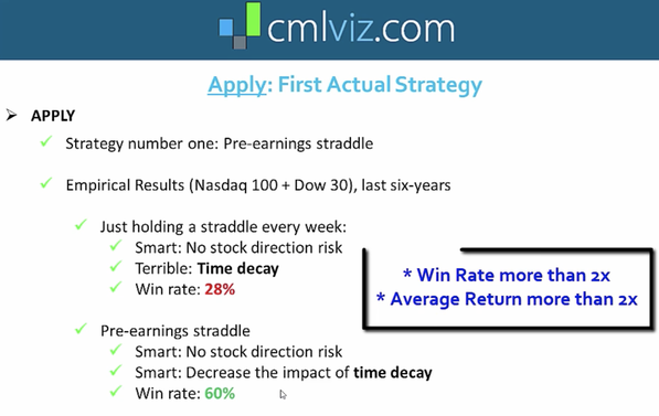
Screenshot from CMLviz video claiming pre-earnings staddle win rate of 60% on NASDAQ 100 and DOW 30 over the last six years. https://vimeo.com/255317960
In what follows, I rigorously backtest a pre-earnings straddle applied to all companies in the DOW 30 and NASDAQ 100 during the last six years (01/01/12 - 01/01/18). To my surprise, I find that it is indeed a winning strategy over this time period with an average return of +2% per straddle. In addition, I find a win rate of 43% which supports the notion that pre-earnings straddles lose more often than they win but the average return per win is greater in magnitude than that of a loss.
The Data Set
The data set for this study is the entire NASDAQ 100 + DOW 30 over the last six years (01/01/12 - 01/01/18). The reason for this choice is two-fold. First, I would like to be as general as possible, hence the use of a large composite index and time frame. And second, I would like to benchmark my results against the only testable claim about pre-earnings straddles from CMLviz, namely, that pre-earnings straddles have a win rate of 60% on this data set.
Data download
The raw data for this analysis was downloaded using CML Trade Machine and can be found here. For each company, the program was set to open an at-the-money straddle 7 days before earnings and close the straddle 1 day before earnings for every possible earnings report in the backtest's time frame. The expiry for the straddle was 7 days. In addition, 40% stops were applied, which means straddles should close early if 40% gains or losses were met. The reason for these choices was to create a pre-earnings straddle that matches CMLviz as best as possible. No trading fees or additional thresholds were applied. A sample of what the cleaned data frame looks like is shown below and is available for download here .
The raw data for this analysis was downloaded using CML Trade Machine and can be found here. For each company, the program was set to open an at-the-money straddle 7 days before earnings and close the straddle 1 day before earnings for every possible earnings report in the backtest's time frame. The expiry for the straddle was 7 days. In addition, 40% stops were applied, which means straddles should close early if 40% gains or losses were met. The reason for these choices was to create a pre-earnings straddle that matches CMLviz as best as possible. No trading fees or additional thresholds were applied. A sample of what the cleaned data frame looks like is shown below and is available for download here .
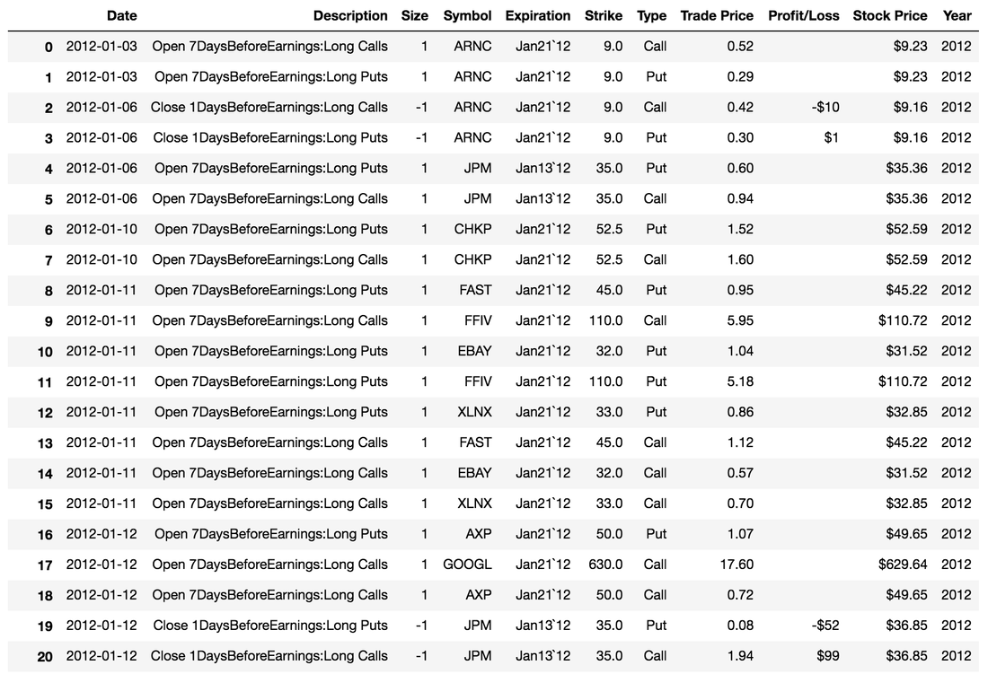
Example slice showing what the backtesting data frame looks like.
Creating the annual index
What exactly is meant by the composite index "NASDAQ 100 + DOW 30" requires a bit more clarification, as the composition of the index changes with time. To this end, I define the index for a given year as the union of all companies that were a part of either the NASDAQ 100 or DOW 30 for any amount of time that year. For example, if company A replaced company B in the NASDAQ 100 in 2016, both A and B will be a part of our composite index for 2016 (but only B will likely remain in the 2017 index). This would result in slightly more than 130 companies in the index each year if not for the fact that there are usually a few companies each year that are a part of both indices (DOW and NASDAQ). The result is a composite index of size 127, 129, 132, 134, 132, and 129 for the years 2012-2017 respectively. A full list of the companies in each index can be found here.
Missing data
The last important thing to note about the data set is that CML Trade Machine only provides historical data for companies with a current ticker. This means data was unobtainable for companies that were once a part of the NASDAQ 100 or DOW 30 but have since gone private, merged, or trade under a new symbol. Naturally, the further back in time we go the more of a problem this is. Fortunately, however, we maintain relatively high coverage for all years in the index (87%, 89%, 89%, 93%, 97% 98%, respectively). A full list of missing data and the corresponding reasons can be found here.
Backtesting
General design
Our backtest is designed as follows. First, we create a hypothetical account with an initial capital of $10M. Then, we step through time and apply a fixed bet to each pre-earnings straddle in our data frame. We keep track of the account value and the straddle results as we go, which serves as the basis for further analysis. The entire code used to perform the backtest and analyze the results can be found here.
Initial capital and bet size
The choice of initial capital must be made in tandem with the bet size. If the bet size is too large, stochastic effects can quickly drain the account even if we have a winning strategy. For this reason, we want the initial capital to be many times the size of the bet.
In addition, the bet size must be many times the cost of an individual straddle (which is typically a few hundred dollars). This is so we can bet approximately the same amount at each straddle opportunity, despite differences between companies/time in the cost of a single straddle. For example, if a straddle costs $150 and we want to bet a fixed amount of $200, there is no way to do this since the bet must be an integer multiple of the straddle cost (i.e. $150, $300, $450,...). If instead, we bet a large amount, say $10,000, then buying 67 straddles at $150 puts us within 1% of our target. Thus, big bets relative to the cost of the straddle allow us to safely ignore biases introduced by the cost of individual straddles. In practice, we assume we are always able to bet exactly the desired amount (i.e. one can by fractional contracts) which is a safe assumption given that the bet size is much larger than the size of the straddle.
We also choose to use fixed bets rather than adaptive bets. This is primarily for simplicity, as adaptive bets are a much smarter way to invest. In order to create a good adaptive betting strategy, however, one must understand the expected distribution of returns, which we do not know a priori.
For these reasons, we backtest fixed bet sizes of $10K, $100K, and $300K. In terms of initial account value, these bets correspond to 0.1%, 1%, and 3%, respectively.
Results
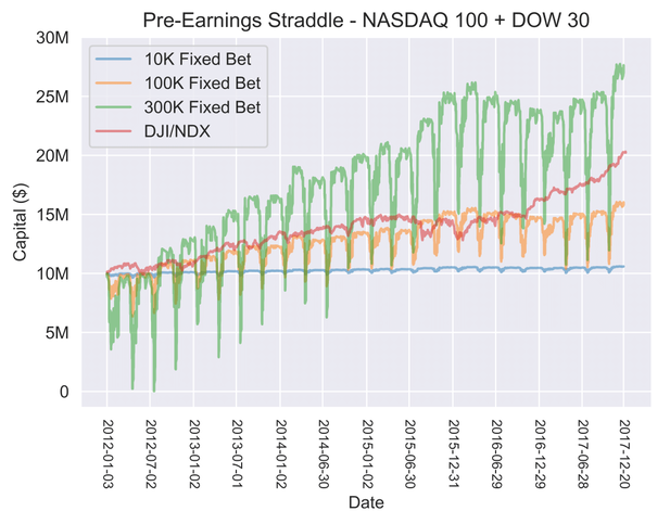
Pre-earnings straddle backtest results for three different bet sizes compared to the underlying market value over this same time frame (shown in red). Oscillations are explained in text.
Backtest
The primary results of our backtest are shown in the time series of account value above. From this, the following conclusions can be drawn:
- Pre-earnings straddles are a winning strategy
For all three bet sizes, our account value clearly increased over time, which means pre-earnings straddles are a winning strategy for this historical data set. Of course, this trend is superimposed over drastic oscillations in account value caused by the upfront cost of betting on numerous pre-earnings straddles at once (more on this later).
- Returns are proportional to bet size
Even though we have a winning strategy, we must bet enough to beat the market (shown in red in the figure above). Both the $10K and the $100K bet fail to do this, while the $300K bet succeeds. Given an expected return P per pre-earnings straddle, we can expect to make PB ($) every time we place a bet of size B ($). If we place N bets of this size, then our expected gain is NPB ($) . Thus, the increase in account value is directly proportional to the bet size B.
- Large bets can freeze your account
If the bet size is too large, losses can cause your account to drop below the minimum amount to place a bet. For example, the very first pre-earnings straddle in our backtest (ARNC, 01/03/12) resulted in an 11% loss; if we were to set a fixed bet of $10M per straddle, our new account value would be $8.9M and we would be unable to place another bet due to insufficient funds.
Similarly, accounts can freeze temporarily if we can't absorb the cost of opening many contracts at once. For example, in July 2012, we were unable to place some $300K bets because our account would drop below $300K due to many open contracts. When these contracts were closed, however, the account would bounce back over $300K and we could resume normal trading. The amount of trades lost during this window, however, may or may not have been worth the gains from increased bet size.
- Adaptive bets are the ideal strategy
Given the previous points, there is clearly a tradeoff between the amount you bet per straddle and the number of straddles you can bet on. In general, we would like to increase our bet size to be as large as possible while still betting as frequently as possible. Under the assumption that the distribution of returns is stable with time, it should be possible to calculate an adaptive strategy that optimally solves this problem and outperforms any fixed betting strategy.
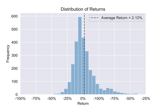
Distribution of returns
The distribution of returns (shown below) is the heart and soul of our statistical analysis. It is the mean of this distribution that tells us the expected return is 2.12% per straddle and the variance of this distribution is what will allow us to create safe adaptive betting strategies in the future. In addition, we can simulate what happens when we apply pre-earnings straddles outside our backtesting window simply by assuming we are drawing from this distribution.
The primary results of our backtest are shown in the time series of account value above. From this, the following conclusions can be drawn:
- Pre-earnings straddles are a winning strategy
For all three bet sizes, our account value clearly increased over time, which means pre-earnings straddles are a winning strategy for this historical data set. Of course, this trend is superimposed over drastic oscillations in account value caused by the upfront cost of betting on numerous pre-earnings straddles at once (more on this later).
- Returns are proportional to bet size
Even though we have a winning strategy, we must bet enough to beat the market (shown in red in the figure above). Both the $10K and the $100K bet fail to do this, while the $300K bet succeeds. Given an expected return P per pre-earnings straddle, we can expect to make PB ($) every time we place a bet of size B ($). If we place N bets of this size, then our expected gain is NPB ($) . Thus, the increase in account value is directly proportional to the bet size B.
- Large bets can freeze your account
If the bet size is too large, losses can cause your account to drop below the minimum amount to place a bet. For example, the very first pre-earnings straddle in our backtest (ARNC, 01/03/12) resulted in an 11% loss; if we were to set a fixed bet of $10M per straddle, our new account value would be $8.9M and we would be unable to place another bet due to insufficient funds.
Similarly, accounts can freeze temporarily if we can't absorb the cost of opening many contracts at once. For example, in July 2012, we were unable to place some $300K bets because our account would drop below $300K due to many open contracts. When these contracts were closed, however, the account would bounce back over $300K and we could resume normal trading. The amount of trades lost during this window, however, may or may not have been worth the gains from increased bet size.
- Adaptive bets are the ideal strategy
Given the previous points, there is clearly a tradeoff between the amount you bet per straddle and the number of straddles you can bet on. In general, we would like to increase our bet size to be as large as possible while still betting as frequently as possible. Under the assumption that the distribution of returns is stable with time, it should be possible to calculate an adaptive strategy that optimally solves this problem and outperforms any fixed betting strategy.
Distribution of returns
The distribution of returns (shown below) is the heart and soul of our statistical analysis. It is the mean of this distribution that tells us the expected return is 2.12% per straddle and the variance of this distribution is what will allow us to create safe adaptive betting strategies in the future. In addition, we can simulate what happens when we apply pre-earnings straddles outside our backtesting window simply by assuming we are drawing from this distribution.
Win rate
Not to be confused with the average return, the win rate for a given company is the number of times a straddle was successful for that company divided by the total number of times a straddle was applied for that company. The average win rate is then the mean of this distribution, which is 42.63%. Of course, one can also calculate the average win rate by tallying the total number of wins for all companies divided by the total number of straddles applied. This method is a more natural definition, as it puts all straddles on equal footing. In our case, however, both methods yield roughly the same result (42.63% and 42.74% respectively).
Not to be confused with the average return, the win rate for a given company is the number of times a straddle was successful for that company divided by the total number of times a straddle was applied for that company. The average win rate is then the mean of this distribution, which is 42.63%. Of course, one can also calculate the average win rate by tallying the total number of wins for all companies divided by the total number of straddles applied. This method is a more natural definition, as it puts all straddles on equal footing. In our case, however, both methods yield roughly the same result (42.63% and 42.74% respectively).
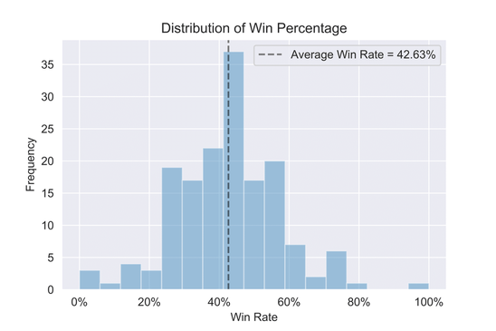
It is interesting to note that the win rate is less than 50% but average returns are still greater than 0%. This means that we lose more often than we win but asymmetric returns on wins more than compensate for losses. There is of course an inherent asymmetry in pre-earnings straddles in the form of bounded losses vs unbounded gains (the most you can lose is your premium while the most you can go is unbounded) but this does not imply a higher returns per win than loss.
Oscillations
As mentioned before, the steep decline in account value each quarter is due to the upfront cost of placing a large number of bets at the same time. This becomes clear when we plot the marginal pdf for one of the betting strategies, as shown below. Spikes in the marginal PDF correspond to a high density of data points, representing the opening/closing of a large volume of trades. At the beginning of each quarter, a large number of trades open (spikes in the marginal PDF) which, in turn, causes the account value to drop. Over the following week, the account value climbs back up as these trades close.
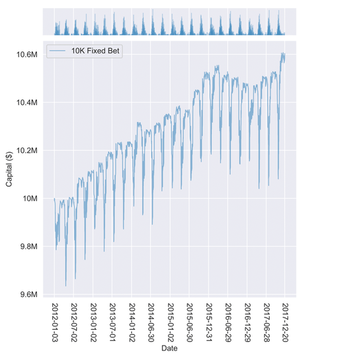
Backtest results for the 10K fixed bet strategy with the marginal PDF shown in the top panel. The steep drops in account value correspond to spikes in the marginal PDF, meaning lots of trades were placed.
Discussion
CML claim not supported
The choice of our backtesting parameters was in part to test the claim by CMLviz that pre-earnings straddles have an empirical win rate of 60%. Using the same index over the same time frame, we calculate a win rate of 43%, which differs substantially from what is claimed. There may be a discrepancy in backtest parameters that can account for this difference, but without knowing what other parameters were used by CML it is impossible to know if this is the case.
Why did we get -8% returns in Part 1?
In Part 1 of this post, we applied a pre-earnings straddle to 20 companies randomly drawn from the S&P 100 in 2016 and found an expected return of -8%. In Part 2, we applied a similar analysis to the DOW 30 + NASDAQ 100 and found an expected return of +2%. What accounts for this difference?
Had the 20 stocks in Part 1 been a part of the index used in Part 2 it would be easy to double check whether returns for these companies were indeed -8% in 2016. Unfortunately, only 8 of the 20 companies from the S&P in Part 1 are a part of the NASDAQ 100 + DOW 30 used in Part 2. For these 8 companies, however, the average return was -5% which suggests that the specific companies used in Part 1 actually do behave statistically differently than the companies used in Part 2.
To test this hypothesis, we can randomly draw 80 samples, representing the 80 straddles in Part 1, from our win rate distribution found in Part 2 and calculate the expected return. If we then repeat this many times, we get a distribution of average returns, which allows us to see how anomalous the results from Part 1 are if we assume the companies are from the same distribution as Part 2. As the figure below shows, the expected return from Part 1 is extremely anomalous relative to the distribution of returns in Part 2. Quantitatively, this means we can reject the null hypothesis with 4.5 sigma confidence (2 sided p-value = 6.8e-6) which qualitatively implies the data used in Part 1 is not a small sample anomaly, but rather, comes from a different distribution altogether.
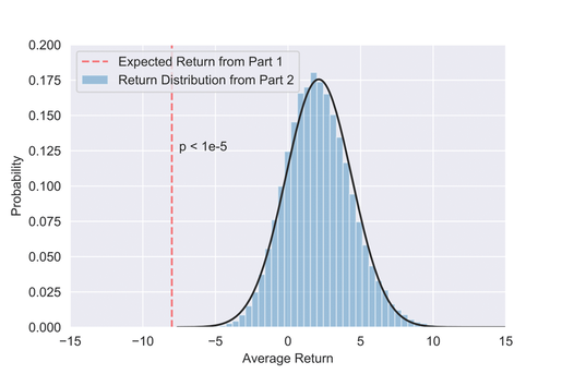
Distribution of average returns under the null hypothesis that the data in Part 1 is drawn from the return distribution in Part 2. The red line shows it is extremely unlikely our data from Part 1 was drawn from this distribution (p < 1e-5).
Perhaps the difference is also due in part to 2016 being an anomalous year relative to other years. We can address this hypothesis by looking at how anomalous our result from Part 1 is relative to the distribution of returns from Part 2 in 2016. As it turns out, 2016 was indeed a bad year (average return of -1% per straddle) but not bad enough to explain the discrepancy (z-score of -3.5, p-value of 0.0003). This reinforces the conclusion that the companies in Part 1 are indeed drawn from a statistically different distribution of returns than the companies in Part 2.
Are all companies the same?
Based on the results of the previous paragraph, we would like to formally test whether there are in fact certain companies for which pre-earnings straddles are more or less well suited. These atypical companies should show anomalous historical win percentages. The null hypothesis, however, is that these anomalous win percentages are just statistical fluctuations due to random chance.
If all companies are independently drawn from the same underlying distribution, then we would expect the distribution of win percentages for companies to be binomially distributed. As the figure below shows, this is not the case. Using the Kolmogorov-Smirnov statistic, we can reject the null hypothesis that all companies are drawing from a binomial distribution with 3-sigma confidence. This does not necessarily imply there are companies with abnormally high or low win percentages, but it does imply the individual results of pre-earnings straddles are not being drawn independently from a binomial distribution - a useful first step toward understanding the true distribution in question.
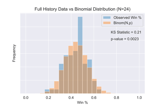
Observed win percentage for companies with 24 straddles (blue) compared to a binomial distribution (orange) with N=24 and p given by the average observed win percentage. KS test shows the probability they are drawn from the same distribution to be 0.0023.
Lingering Concerns
There are still several big concerns that I would like to address before concluding whether or not I recommend a pre-earnings straddle.
Anomalous delta values and >40% returns using CML Trade Machine
My primary concern with the results has to do with using CML Trade Machine to generate the data for the backtest. In general, CML Trade Machine appears to work quite well but close inspection of the data revealed a few potential problems. First, the 40% limit on gains only sometimes closed the straddle. As you can see in the distribution of returns, there are many straddles with returns greater than 40% despite setting a 40% limit. I double checked the data coming from CML Trade Machine on these straddles and confirmed that it was being generated without throwing any errors (e.g. ADI opened a straddle at $2.30 on 2/10/15 and closed the straddle at $4.15 on 2/17/15).
Similarly, the delta values of pre-earnings straddles were sometimes very far from 50. Theoretically, delta values should be around 50 when opening at-the-money calls or puts but, when I manually inspected the data this was not always the case. Unfortunately, delta values are not included in the data downloads (they have to be copied by hand) so I have not yet pursued this any further.
My guess is that the historical data used by CML Trade Machine is sparse in certain regions of the parameter space and the program is designed to grab the closest trade possible to what is desired. This would explain why it isn't always possible to get 50 delta straddles and close trades at exactly 40% gains/losses. If this is the case, however, there are likely important downstream consequences and it is worth testing pre-earnings straddles using data generated independently from CML. This is also good practice in general.
Stability of Returns
By definition, a winning strategy has an average return greater than 0%. Our backtest showed the distribution of returns to have a mean of +2% over the last six years. However, we also saw that 2016 had a negative expected return, which hints at the fact the return distribution fluctuates with time. Similarly, we also saw that the results from Part 1 could not be fit by the return distribution from Part 2, which implies the return distribution is sensitive to the choice of companies in the index. Taken together, this implies we may not always be justified in assuming returns based on historical data will continue to hold in the future. This is by far the most serious worry I would have when applying this strategy.
Conclusion
Given the preliminary results from Part 1, I am genuinely surprised that a pre-earnings straddle worked historically in Part 2. Our backtest found expected returns of +2% per straddle, which means we should bet as big and as often as possible with the caveat that betting too big may actually prevent us from betting often. In light of this, the ideal betting strategy is clearly adaptive, rather than fixed, and should be crafted using the distribution of returns and a better understanding of how this distribution fluctuates with time and choice of index. Before simulating this, however, it is important to address why the data from CML Trade Machine sometimes had delta values far from 50 when opening straddles and why straddles sometimes closed well outside the 40% stop. To this end, an analysis using independent data is warranted. Such an analysis would be a welcome addition to the current study, which, to date, is the only publicly available backtest of a general pre-earnings straddle.
 RSS Feed
